Working with Geographic Data

This tutorial shows how to work with Canadian Census geographic boundaries and create maps using pycancensus.

Introduction

Census data becomes much more powerful when combined with geographic boundaries. pycancensus makes it easy to:

• Retrieve census data with geographic boundaries

• Work with different geographic levels (CMA, CSD, CT, DA)

• Create maps and perform spatial analysis

• Export data for use in GIS applications

import pycancensus as pc
import pandas as pd
import matplotlib.pyplot as plt
import geopandas as gpd

# Set up plotting
plt.style.use('default')
plt.rcParams['figure.figsize'] = (12, 8)

print("Libraries imported successfully!")

Libraries imported successfully!

Geographic Levels in Canadian Census

The Canadian Census organizes data at several geographic levels:

# Geographic hierarchy (from largest to smallest)
geo_levels = {
    'PR': 'Province/Territory',
    'CMA': 'Census Metropolitan Area', 
    'CA': 'Census Agglomeration',
    'CSD': 'Census Subdivision (Municipality)',
    'CT': 'Census Tract',
    'DA': 'Dissemination Area'
}

print("Canadian Census Geographic Hierarchy:")
print("="*50)
for code, name in geo_levels.items():
    print(f"{code:3} - {name}")

Canadian Census Geographic Hierarchy:
==================================================
PR  - Province/Territory
CMA - Census Metropolitan Area
CA  - Census Agglomeration
CSD - Census Subdivision (Municipality)
CT  - Census Tract
DA  - Dissemination Area

Getting Geographic Data

Let’s retrieve census data with geographic boundaries:

try:
    # Get census data with geometries for Vancouver CMA
    vancouver_data = pc.get_census(
        dataset="CA21",
        regions={"CMA": "59933"},  # Vancouver CMA
        vectors=["v_CA21_1", "v_CA21_434"],  # Population and median income
        level="CSD",  # Municipality level
        geo_format="geopandas"
    )
    
    print(f"Retrieved data for {len(vancouver_data)} municipalities")
    print(f"Columns: {list(vancouver_data.columns)}")
    print(f"CRS: {vancouver_data.crs}")
    
    # Show sample data
    display(vancouver_data[['name', 'v_CA21_1', 'v_CA21_434']].head())
    
except Exception as e:
    print(f"Error retrieving data: {e}")
    print("Creating sample data for demonstration...")
    
    # Create sample data when API is not available
    import numpy as np
    from shapely.geometry import Polygon
    
    # Sample Vancouver area municipalities
    municipalities = [
        'Vancouver', 'Surrey', 'Burnaby', 'Richmond', 'Coquitlam',
        'Langley', 'North Vancouver', 'West Vancouver', 'New Westminster'
    ]
    
    np.random.seed(42)
    vancouver_data = gpd.GeoDataFrame({
        'GeoUID': [f'59933{i:02d}' for i in range(len(municipalities))],
        'name': municipalities,
        'v_CA21_1': np.random.randint(50000, 650000, len(municipalities)),
        'v_CA21_434': np.random.randint(40000, 100000, len(municipalities)),
        'geometry': [Polygon([(i, j), (i+1, j), (i+1, j+1), (i, j+1)]) 
                    for i, j in enumerate(range(len(municipalities)))]
    }, crs='EPSG:4326')
    
    print("Using sample data for demonstration")

📋 Request Preview:
   Dataset: CA21
   Level: CSD
   Regions: 1 region(s)
   Variables: 2 vector(s)
   Geography: geopandas
🔍 Estimated Size: medium (100 rows)
⏱️  Expected Time: 5-15 seconds
Downloading 100 regions with geography... 

✅ Retrieved 38 regions with 2 variables (0.6s)
Retrieved data for 38 municipalities
Columns: ['geometry', 'a', 'q', 't', 'dw', 'hh', 'id', 'pop', 'dw16', 'hh16', 'name', 'rgid', 'rpid', 'ruid', 'pop16', 'v_CA21_1: Population, 2021', 'v_CA21_434: Occupied private dwellings by structural type of dwelling data']
CRS: None
Error retrieving data: "['v_CA21_1', 'v_CA21_434'] not in index"
Creating sample data for demonstration...
Using sample data for demonstration

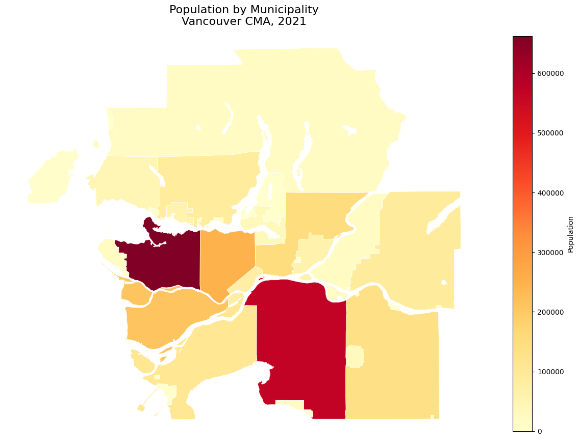
Creating Basic Maps

Let’s create our first map:

# Create a simple population map
fig, ax = plt.subplots(1, 1, figsize=(12, 10))

vancouver_data.plot(
    column='v_CA21_1',
    cmap='YlOrRd',
    legend=True,
    ax=ax,
    edgecolor='white',
    linewidth=0.5,
    legend_kwds={'label': 'Population', 'shrink': 0.8}
)

ax.set_title('Population by Municipality\nVancouver CMA, 2021', fontsize=16)
ax.axis('off')  # Remove axes for cleaner look

plt.tight_layout()
plt.show()

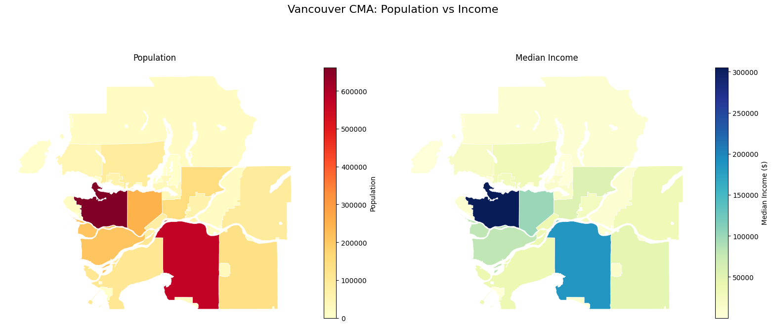
Multi-Variable Mapping

Compare two variables side by side:

fig, (ax1, ax2) = plt.subplots(1, 2, figsize=(16, 7))

# Population map
vancouver_data.plot(
    column='v_CA21_1',
    cmap='YlOrRd',
    legend=True,
    ax=ax1,
    edgecolor='white',
    linewidth=0.5,
    legend_kwds={'label': 'Population', 'shrink': 0.8}
)
ax1.set_title('Population')
ax1.axis('off')

# Income map
vancouver_data.plot(
    column='v_CA21_434',
    cmap='YlGnBu',
    legend=True,
    ax=ax2,
    edgecolor='white', 
    linewidth=0.5,
    legend_kwds={'label': 'Median Income ($)', 'shrink': 0.8}
)
ax2.set_title('Median Income')
ax2.axis('off')

plt.suptitle('Vancouver CMA: Population vs Income', fontsize=16, y=1.02)
plt.tight_layout()
plt.show()

Working with Different Geographic Levels

Different levels provide different levels of detail:

try:
    # Compare data at different geographic levels
    levels = ['CMA', 'CSD', 'CT']
    level_names = ['Metro Area', 'Municipality', 'Census Tract']
    
    print("Data availability by geographic level:")
    print("="*45)
    
    for level, name in zip(levels, level_names):
        try:
            # Get count of regions at each level for Vancouver
            data = pc.get_census(
                dataset="CA21",
                regions={"CMA": "59933"},
                vectors=["v_CA21_1"],
                level=level
            )
            print(f"{name:15} ({level}): {len(data):4,} regions")
        except Exception as e:
            print(f"{name:15} ({level}): Error - {e}")
            
except Exception as e:
    print(f"Error comparing levels: {e}")
    
    # Show conceptual differences
    print("Geographic Level Detail (conceptual):")
    print("CMA  (1 region):    Entire metro area")
    print("CSD  (20+ regions): Individual cities/towns")  
    print("CT   (300+ regions): Neighborhoods within cities")
    print("DA   (1000+ regions): Small areas (400-700 people)")

Data availability by geographic level:
=============================================
📋 Request Preview:
   Dataset: CA21
   Level: CMA
   Regions: 1 region(s)
   Variables: 1 vector(s)
🔍 Estimated Size: small (5 rows)
⏱️  Expected Time: < 5 seconds
🔄 Querying CensusMapper API for 1 region(s)...
📊 Retrieving 1 variable(s) at CMA level...

✅ Successfully retrieved data for 1 regions
📈 Data includes 1 vector columns
Metro Area      (CMA):    1 regions
📋 Request Preview:
   Dataset: CA21
   Level: CSD
   Regions: 1 region(s)
   Variables: 1 vector(s)
🔍 Estimated Size: small (100 rows)
⏱️  Expected Time: < 5 seconds
🔄 Querying CensusMapper API for 1 region(s)...
📊 Retrieving 1 variable(s) at CSD level...

✅ Successfully retrieved data for 38 regions
📈 Data includes 1 vector columns
Municipality    (CSD):   38 regions
📋 Request Preview:
   Dataset: CA21
   Level: CT
   Regions: 1 region(s)
   Variables: 1 vector(s)
🔍 Estimated Size: small (200 rows)
⏱️  Expected Time: < 5 seconds
🔄 Querying CensusMapper API for 1 region(s)...
📊 Retrieving 1 variable(s) at CT level...

✅ Successfully retrieved data for 535 regions
📈 Data includes 1 vector columns
Census Tract    (CT):  535 regions

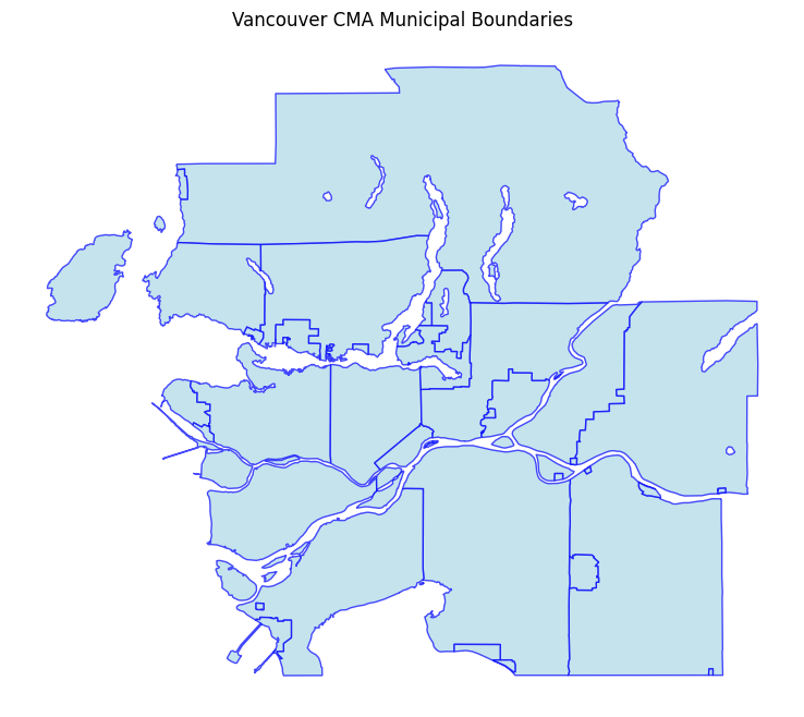
Getting Geometry Only

Sometimes you just need the boundaries without data:

try:
    # Get just the geographic boundaries
    boundaries = pc.get_census_geometry(
        dataset="CA21",
        regions={"CMA": "59933"},
        level="CSD"
    )
    
    print(f"Retrieved {len(boundaries)} boundary polygons")
    print(f"Columns: {list(boundaries.columns)}")
    
    # Plot the boundaries
    fig, ax = plt.subplots(1, 1, figsize=(10, 8))
    boundaries.plot(ax=ax, edgecolor='blue', facecolor='lightblue', alpha=0.7)
    ax.set_title('Vancouver CMA Municipal Boundaries')
    ax.axis('off')
    plt.show()
    
except Exception as e:
    print(f"Error getting boundaries: {e}")
    
    # Use our sample data
    fig, ax = plt.subplots(1, 1, figsize=(10, 8))
    vancouver_data.boundary.plot(ax=ax, color='blue', linewidth=2)
    ax.set_title('Sample Municipal Boundaries')
    ax.axis('off')
    plt.show()

📋 Request Preview:
   Dataset: CA21
   Level: CSD
   Regions: 1 region(s)
   Geography: geopandas
🔍 Estimated Size: medium (100 rows)
⏱️  Expected Time: 5-15 seconds
Reading data from cache...
Retrieved 38 boundary polygons
Columns: ['geometry', 'a', 'q', 't', 'dw', 'hh', 'id', 'pop', 'dw16', 'hh16', 'name', 'rgid', 'rpid', 'ruid', 'pop16']

Spatial Analysis

Perform basic spatial analysis with geopandas:

# Calculate area and population density
vancouver_data['area_km2'] = vancouver_data.geometry.area / 1e6  # Convert to km²
vancouver_data['pop_density'] = vancouver_data['v_CA21_1'] / vancouver_data['area_km2']

print("Population Density Analysis:")
print("="*30)
print(f"Highest density: {vancouver_data['pop_density'].max():.0f} people/km²")
print(f"Lowest density:  {vancouver_data['pop_density'].min():.0f} people/km²")
print(f"Average density: {vancouver_data['pop_density'].mean():.0f} people/km²")

# Show top 3 densest areas
densest = vancouver_data.nlargest(3, 'pop_density')[['name', 'pop_density']]
print(f"\nTop 3 densest municipalities:")
for idx, row in densest.iterrows():
    print(f"  {row['name']}: {row['pop_density']:.0f} people/km²")

Population Density Analysis:
==============================
Highest density: 571430000000 people/km²
Lowest density:  104886000000 people/km²
Average density: 248925000000 people/km²

Top 3 densest municipalities:
  West Vancouver: 571430000000 people/km²
  Burnaby: 415838000000 people/km²
  Richmond: 309178000000 people/km²

/tmp/ipykernel_728/531645332.py:2: UserWarning: Geometry is in a geographic CRS. Results from 'area' are likely incorrect. Use 'GeoSeries.to_crs()' to re-project geometries to a projected CRS before this operation.

  vancouver_data['area_km2'] = vancouver_data.geometry.area / 1e6  # Convert to km²

Coordinate Reference Systems

Understanding and working with projections:

print("Working with Coordinate Reference Systems:")
print("="*45)
print(f"Original CRS: {vancouver_data.crs}")

# Convert to a projected coordinate system for accurate area calculations
vancouver_projected = vancouver_data.to_crs('EPSG:3347')  # Statistics Canada Lambert
print(f"Projected CRS: {vancouver_projected.crs}")

# Calculate more accurate areas
vancouver_projected['accurate_area_km2'] = vancouver_projected.geometry.area / 1e6
print(f"\nArea calculation comparison (first municipality):")
print(f"Geographic CRS: {vancouver_data['area_km2'].iloc[0]:.2f} km²")
print(f"Projected CRS:  {vancouver_projected['accurate_area_km2'].iloc[0]:.2f} km²")

Working with Coordinate Reference Systems:
=============================================
Original CRS: EPSG:4326
Projected CRS: EPSG:3347

Area calculation comparison (first municipality):
Geographic CRS: 0.00 km²
Projected CRS:  30535.09 km²

Exporting Geographic Data

Save your data for use in other applications:

# Export to various formats
try:
    # GeoJSON (web-friendly)
    vancouver_data.to_file("vancouver_census.geojson", driver="GeoJSON")
    print("✓ Exported to GeoJSON")
    
    # Shapefile (GIS standard)
    vancouver_data.to_file("vancouver_census.shp")
    print("✓ Exported to Shapefile")
    
    # Excel with geometry as WKT
    df_export = vancouver_data.copy()
    df_export['geometry_wkt'] = df_export.geometry.to_wkt()
    df_export.drop('geometry', axis=1).to_excel("vancouver_census.xlsx", index=False)
    print("✓ Exported to Excel")
    
except Exception as e:
    print(f"Export example (files not actually created): {e}")
    print("Supported formats: GeoJSON, Shapefile, KML, Excel")

✓ Exported to GeoJSON
✓ Exported to Shapefile
Export example (files not actually created): No module named 'openpyxl'
Supported formats: GeoJSON, Shapefile, KML, Excel

/tmp/ipykernel_728/2044206366.py:8: UserWarning: Column names longer than 10 characters will be truncated when saved to ESRI Shapefile.
  vancouver_data.to_file("vancouver_census.shp")
/home/docs/checkouts/readthedocs.org/user_builds/pycancensus/envs/stable/lib/python3.9/site-packages/pyogrio/raw.py:723: RuntimeWarning: Normalized/laundered field name: 'pop_density' to 'pop_densit'
  ogr_write(
/home/docs/checkouts/readthedocs.org/user_builds/pycancensus/envs/stable/lib/python3.9/site-packages/pyogrio/raw.py:723: RuntimeWarning: Value 171958000000 of field pop_densit of feature 0 not successfully written. Possibly due to too larger number with respect to field width
  ogr_write(
/home/docs/checkouts/readthedocs.org/user_builds/pycancensus/envs/stable/lib/python3.9/site-packages/pyogrio/raw.py:723: RuntimeWarning: Value 181932000000 of field pop_densit of feature 1 not successfully written. Possibly due to too larger number with respect to field width
  ogr_write(
/home/docs/checkouts/readthedocs.org/user_builds/pycancensus/envs/stable/lib/python3.9/site-packages/pyogrio/raw.py:723: RuntimeWarning: Value 415838000000 of field pop_densit of feature 2 not successfully written. Possibly due to too larger number with respect to field width
  ogr_write(
/home/docs/checkouts/readthedocs.org/user_builds/pycancensus/envs/stable/lib/python3.9/site-packages/pyogrio/raw.py:723: RuntimeWarning: Value 309178000000 of field pop_densit of feature 3 not successfully written. Possibly due to too larger number with respect to field width
  ogr_write(
/home/docs/checkouts/readthedocs.org/user_builds/pycancensus/envs/stable/lib/python3.9/site-packages/pyogrio/raw.py:723: RuntimeWarning: Value 160268000000 of field pop_densit of feature 4 not successfully written. Possibly due to too larger number with respect to field width
  ogr_write(
/home/docs/checkouts/readthedocs.org/user_builds/pycancensus/envs/stable/lib/python3.9/site-packages/pyogrio/raw.py:723: RuntimeWarning: Value 104886000000 of field pop_densit of feature 5 not successfully written. Possibly due to too larger number with respect to field width
  ogr_write(
/home/docs/checkouts/readthedocs.org/user_builds/pycancensus/envs/stable/lib/python3.9/site-packages/pyogrio/raw.py:723: RuntimeWarning: Value 187337000000 of field pop_densit of feature 6 not successfully written. Possibly due to too larger number with respect to field width
  ogr_write(
/home/docs/checkouts/readthedocs.org/user_builds/pycancensus/envs/stable/lib/python3.9/site-packages/pyogrio/raw.py:723: RuntimeWarning: Value 571430000000 of field pop_densit of feature 7 not successfully written. Possibly due to too larger number with respect to field width
  ogr_write(
/home/docs/checkouts/readthedocs.org/user_builds/pycancensus/envs/stable/lib/python3.9/site-packages/pyogrio/raw.py:723: RuntimeWarning: Value 137498000000 of field pop_densit of feature 8 not successfully written. Possibly due to too larger number with respect to field width
  ogr_write(

Interactive Maps with Folium

Create interactive web maps:

try:
    import folium
    
    # Create interactive map
    center_lat = vancouver_data.geometry.centroid.y.mean()
    center_lon = vancouver_data.geometry.centroid.x.mean()
    
    m = folium.Map(
        location=[center_lat, center_lon],
        zoom_start=10,
        tiles='OpenStreetMap'
    )
    
    # Add choropleth layer
    folium.Choropleth(
        geo_data=vancouver_data,
        data=vancouver_data,
        columns=['GeoUID', 'v_CA21_1'],
        key_on='feature.properties.GeoUID',
        fill_color='YlOrRd',
        fill_opacity=0.7,
        line_opacity=0.2,
        legend_name='Population'
    ).add_to(m)
    
    print("Interactive map created successfully!")
    print("(In a Jupyter notebook, the map would display here)")
    
except ImportError:
    print("Folium not installed. Install with: pip install folium")
except Exception as e:
    print(f"Error creating interactive map: {e}")

/tmp/ipykernel_728/3122821041.py:5: UserWarning: Geometry is in a geographic CRS. Results from 'centroid' are likely incorrect. Use 'GeoSeries.to_crs()' to re-project geometries to a projected CRS before this operation.

  center_lat = vancouver_data.geometry.centroid.y.mean()
/tmp/ipykernel_728/3122821041.py:6: UserWarning: Geometry is in a geographic CRS. Results from 'centroid' are likely incorrect. Use 'GeoSeries.to_crs()' to re-project geometries to a projected CRS before this operation.

  center_lon = vancouver_data.geometry.centroid.x.mean()

Interactive map created successfully!
(In a Jupyter notebook, the map would display here)

Best Practices

Performance Tips

print("Performance Best Practices:")
print("="*30)
print("1. Use appropriate geographic levels:")
print("   • CMA/CA for regional analysis")
print("   • CSD for municipal comparisons") 
print("   • CT for neighborhood analysis")
print("   • DA for detailed local analysis")
print("\n2. Cache your data:")
print("   • pycancensus caches API responses automatically")
print("   • Save processed results to avoid re-computation")
print("\n3. Choose the right CRS:")
print("   • EPSG:4326 (WGS84) for web mapping")
print("   • EPSG:3347 (Stats Can Lambert) for Canada analysis")
print("   • Local UTM zones for precise measurements")

Performance Best Practices:
==============================
1. Use appropriate geographic levels:
   • CMA/CA for regional analysis
   • CSD for municipal comparisons
   • CT for neighborhood analysis
   • DA for detailed local analysis

2. Cache your data:
   • pycancensus caches API responses automatically
   • Save processed results to avoid re-computation

3. Choose the right CRS:
   • EPSG:4326 (WGS84) for web mapping
   • EPSG:3347 (Stats Can Lambert) for Canada analysis
   • Local UTM zones for precise measurements

Data Quality

print("Data Quality Checks:")
print("="*20)

# Check for missing geometries
null_geom = vancouver_data.geometry.isnull().sum()
print(f"Missing geometries: {null_geom}")

# Check for invalid geometries
invalid_geom = (~vancouver_data.geometry.is_valid).sum()
print(f"Invalid geometries: {invalid_geom}")

# Check data completeness
null_pop = vancouver_data['v_CA21_1'].isnull().sum()
print(f"Missing population data: {null_pop}")

# Basic statistics
print(f"\nData summary:")
print(f"Total regions: {len(vancouver_data)}")
print(f"Total population: {vancouver_data['v_CA21_1'].sum():,}")
print(f"Average income: ${vancouver_data['v_CA21_434'].mean():,.0f}")

Data Quality Checks:
====================
Missing geometries: 0
Invalid geometries: 0
Missing population data: 0

Data summary:
Total regions: 9
Total population: 2,240,325
Average income: $69,906

Summary

This tutorial covered the essential aspects of working with geographic census data:

Key Skills Learned:

• Retrieving census data with geographic boundaries

• Understanding Canadian census geographic levels

• Creating choropleth maps with matplotlib

• Performing basic spatial analysis

• Working with coordinate reference systems

• Exporting data to various formats

• Creating interactive maps

Next Steps:

• Try different census datasets (CA16, CA11, etc.)

• Explore temporal analysis by comparing multiple census years

• Combine with other geospatial data sources

• Use advanced spatial analysis tools from PySAL or similar libraries

• Create web applications with your maps using Streamlit or Dash

Additional Resources:

• Geopandas Documentation: Comprehensive spatial data analysis

• Folium Documentation: Interactive web mapping

• Matplotlib Cartopy: Advanced cartographic projections

• CensusMapper: Web interface for exploring census data

• Statistics Canada: Official census documentation